Help -- Creating Expressions for Calculated Measure Items

Creating Expressions for Calculated Measure Items

These tables have example expressions that can be used as models when you are setting up expressions for calculated measure items.

Note: If you want to set up views that return YTD data, comparisons of current vs past periods, rolling N periods, previous N periods, etc., do so using regular measure items with time ranges. Examples are in Using Time Ranges vs. Time Hierarchies in Views. If you want to set up a calculated measure item that displays an image, see Display Images for Measure Items.

Calculations with Stratum.Viewer Functions

Type of Calculation & Function

Example

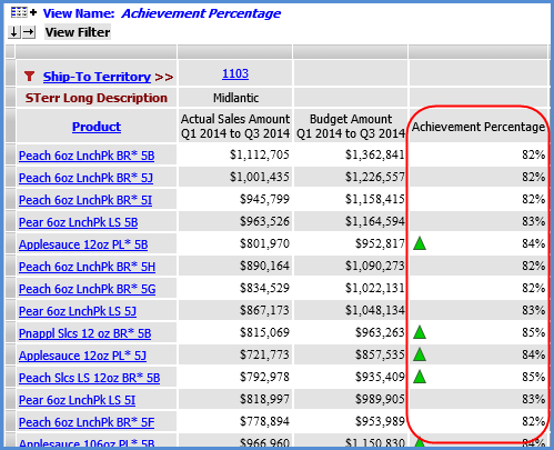
Achievement Percent

Has a built-in divide by zero check to avoid divide by zero errors.

#AchievementPercent([Measures].[Data1 (Actual Sales Sales Amount Q1 2014 to Q3 2014 )], [Measures].[Data2 (Budget Budget Amount Frozen Q1 2014 to Q3 2014)])

Returns the achievement percentage between two measure items -- in this case, the percent of sales achieved in comparison to the budgeted sales.
The expression for this function is Measure Item 1 / Measure Item 2 with a divide by zero check. The divide by zero check will return null if Measure item 2, the divisor, is zero or null.
The expression syntax includes the names (Data1 and Data2) and captions of the specified measure items.
Recommendations: select a percentage Format String and set Total property to None.

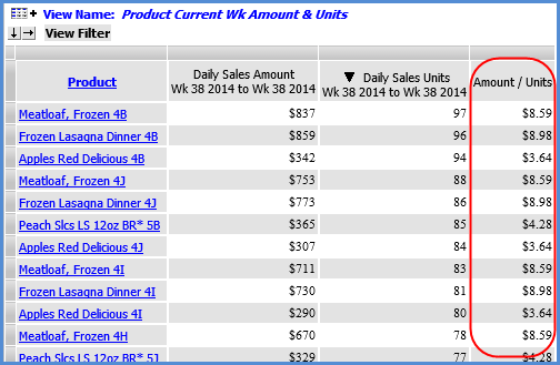
Divide with Zero Check

Has a built-in divide by zero check to avoid divide by zero errors.

#DivideWithZeroCheck([Measures].[Data1 (Daily Sales Amount Wk 38 2014 to Wk 38 2014)], [Measures].[Data2 (Daily Sales Units Wk 38 2014 to Wk 38 2014)])

Divides two numbers with a divide by zero check.
The expression for this function is Measure Item 1 / Measure Item 2 with a divide by zero check. The divide by zero check will return null if Numeric Expression 2, the divisor, is zero or null.
The expression syntax includes the names (Data1 and Data2) and captions of the specified measure items.

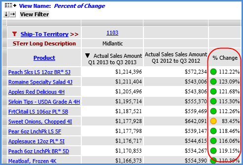
Percent of Change

Has a built-in divide by zero check to avoid divide by zero errors.

#PercentOfChange([Measures].[Data1 (Actual Sales Amount Q1 2013 to Q3 2013)], [Measures].[Data2 (Actual Sales Sales Amount Q1 2012 to Q3 2012)])

Returns the percent of change, also known as the variance percentage, between two measure items or expressions -- in this case, the change between YTD sales for two different years.
The expression for this function is (Measure Item 1 - Measure Item 2) / Measure Item 2 with a divide by zero check. The divide by zero check will return null if Measure item 2, the divisor, is zero or null.
The expression syntax includes the names (Data1 and Data2) and captions of the specified measure items.
Recommendations: select a percentage Format String and set Total property to None.

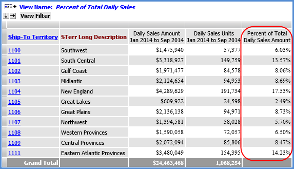
Percent Of Total

#PercentOfTotal([Measures].[Data1 (Daily Sales Amount Jan 2014 to Sep 2014)])

Returns percent of total for the designated measure item, in this case Daily Sales Daily Sales Amount Jan 2014 to Sep 2014 (this caption and the measure item name Data1 are part of the MDX syntax in the expression).
Recommendations: select a percentage Format String.

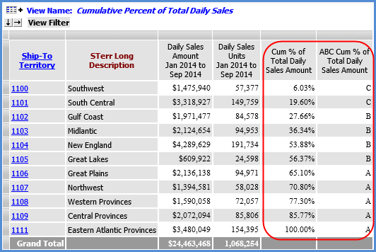
Cumulative Percent Of Total

and

ABC Cumulative Percent Of Total

#CumulativePercentOfTotal([Measures].[Data1 (Daily Sales Amount Jan 2014 to Sep 2014)])

Returns cumulative percent of total for the designated measure item, in this case Daily Sales Amount Jan 2014 to Sep 2014 (this caption and the measure item name Data1 are part of the MDX syntax in the expression).
Recommendations: select a percentage Format String and set Total property to None.

and

#ABCCumulativePercent([Measures].[Data1 (Daily Sales Amount Jan 2014 to Sep 2014)],".65;.25")

Assigns specified ranking values to results of the cumulative percent of total calculation, based on ranges specified in the expression. This expression assigns the following ranks: A for values >= 65%. B for values < 65% and >= 25%, and C for values < 25%.
Recommendations: leave Format String set to None and set Total property to None.

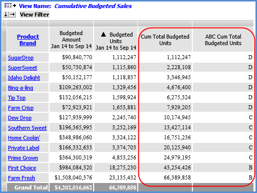
Cumulative Total

and

ABC Cumulative Total

#CumulativeTotal([Measures].[Data2 (Budgeted Units Jan 14 to Sep 14)])

Returns cumulative total for the designated measure item, in this case Budgeted Units Jan 14 to Sep 14 (this caption and the measure item name Data2 are part of the MDX syntax in the expression).
Recommendations: set Format String to the same Format String for the measure item referenced in the expression and set Total property to None.

and

#ABCCumulative([Measures].[Data2 (Budgeted Units Jan 14 to Sep 14)],"75000000.00;35000000.00;10000000.00")

Assigns specified ranking values to results of the cumulative total calculation, based on ranges specified in the expression. This expression assigns the following ranks: A for values >= 75,000,000; B for values < 75,000,000 and >= 35,0000,000; C for values < 35,000,000 and >= 10,000,000; and D for values < 10,000,000.
Recommendations: leave Format set to None and set Total property to None.

Other Types of Calculations

Type of Calculation & Function

Example Expression

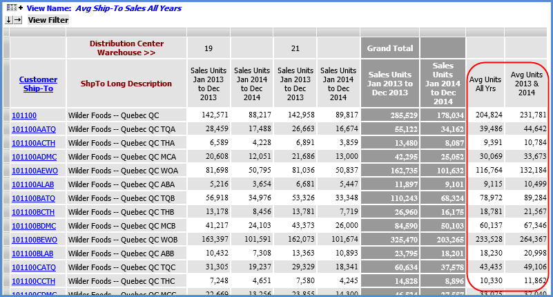
Average

Uses Average numeric function.

Avg({[Time].[Year Months].[Year].members},[Measures].[Actual Sales Sales Units])

Returns average sales units for all years. Expression references the Year level from the Year Months hierarchy and Actual Sales Sales Units measure.
Recommendations: set Type to Distinct Calculated.

and

Avg({[Time].[Year Months].[Year].[2013], [Time].[Year Months].[Year].[2014]},[Measures].[Actual Sales Sales Units])

Returns average sales units for 2013 and 2014. Expression references the 2013 and 2014 members of the Year level from the Year Months hierarchy and Actual Sales Sales Units measure.
Recommendations: set Type to Distinct Calculated.

Difference

[Measures].[Data22 (Act Gross Margin After Rebate)]-[Measures].[Data21 (Std Gross Margin After Rebate)]

Returns difference between the Act Gross Margin After Rebate and Std Gross Margin After Rebate measure items (their captions and the measure item names Data22 and Data21 are part of the MDX syntax in the expression).

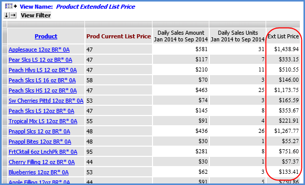
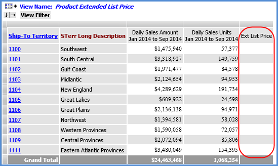
Extended List Price

Uses attribute relationship.

IIF([Product].[Product].CurrentMember.Level.Name="Product",[Product].[Product].Properties("Prod Current List Price") * [Measures].[Data5 (Daily Sales Units Jan 2014 to Sep 2014)], null)

If the Product level is visible, then the following calculation is performed: [Product].[Product].Properties("Prod Current List Price") * [Measures].[Data5 (Daily Sales Units Jan 2014 to Sep 2014)]. This returns the extended list price by multiplying the Prod Current List Price attribute relationship from the Product level by the Daily Sales Units Jan 2014 to Sep 2014 measure. If the Product level is not visible in the view, the calculation will not be performed and a null value (empty cell) will be returned.
The IIF and [Product].[Product].CurrentMember.Level.Name="Product" syntax check for the visibility of the level to which the attribute relationship belongs. The syntax for the measure item used in the expression includes its name (Data5) and caption. The name of the Product level and its hierarchy are included in the syntax.
Recommendation: select a monetary Format String.

Here is the view when the Product level is visible. The calculation is performed.

Here is the view after it has been rearranged. Ship-to Territory is now visible and Product is no longer visible. Null values are returned.

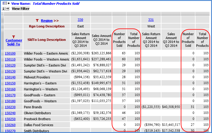
Number of Products Sold and Total Number of Products

Uses Count numeric function and CrossJoin function.

Count(CrossJoin({[UPC Global Number].[UPC Global Number].[UPC Global Number].members},{[Measures].[Data2 (Sales Amount Q3 2014 to Q3 2014)]}),EXCLUDEEMPTY)

and

Count(CrossJoin({[UPC Global Number].[UPC Global Number].[UPC Global Number].members},{[Measures].[Data2 (Sales Amount Q3 2014 to Q3 2014)]}),INCLUDEEMPTY)

The first calculation counts the number of UPC's that have sales. The EXCLUDEEMPTY text is the part of the expression that will exclude UPC members without any sales from the count.
The second calculation counts the total number of UPC's that exist including those with and without sales. The INCLUDEEMPTY text is the part of the expression that will include UPC members without any sales in the count.
The MDX for the UPC Global Number level includes the level name and names of its dimension and hierarchy. The level is analyzed against sales amount values for the third quarter 2014, and the syntax for that part of the expression includes the measure item name (Data2) and caption.
Recommendation: leave the Format String set to None and set Total property to None.

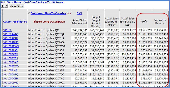
Profit (Sales after Costs)

and

Sales after Returns

Uses Absolute value of a measure item.

[Measures].[Data2 (Actual Sales Sales Amount)]-[Measures].[Data1 (Actual Sales Ext Standard Cost)]

and

[Measures].[Data2 (Actual Sales Sales Amount)]-abs([Measures].[Data4 (Actual Sales Sales Return Amount)])

The first expression returns the profit, the total sales after costs. The syntax for the two measure items used in the calculation includes their captions and names (Data2 and Data1).
The second expression returns the sales after returns. The syntax for the two measure items used in the calculation includes their names (Data2 and Data4) and captions. That part of the expression also uses the Abs function to use the absolute value of returns in the calculation.

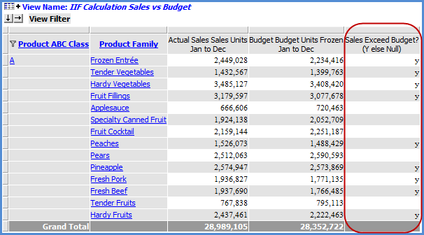
Return Text Value if Condition is Met

Uses IIF function to check for conditions and determine which results to return.

IIF([Measures].[Data22 (Actual Sales Sales Units Jan to Dec)]>[Measures].[Data2 (Budget Budget Units Frozen Jan to Dec)],"y",null)

Uses the IIF function to set up an If/Then/Else scenario. If the specified condition is true, then the first specified value will be returned. Otherwise (else), a null value will be returned. In this case, the condition checked for is whether or not Actual Sales Sales Units are greater than Budget Budget Units Frozen. The calculation returns a "y" (for Yes) if the condition is true. If the condition is not true, the calculation returns a null value (empty cell).
The syntax for the two measure items in both examples includes their names (Data22 and Data2) and captions.
Recommendations: leave Format String set to None. You can use a variety of values for the returned text, such as a letter or word, based on what best suits your view needs. In this case, null is recommended as the second (Else) value to prevent otherwise empty rows or columns from displaying. For example, if a row is hidden by relationship and empty filter because it has no sales or budget data, it would display if you set the second value in the expression to a 0 or "n" because those results would be considered a value by the relationship and empty filter. Using null as we did keeps results in an empty cell for such rows and therefore the rows will remain hidden. See also Using Relationship and Empty Filters.

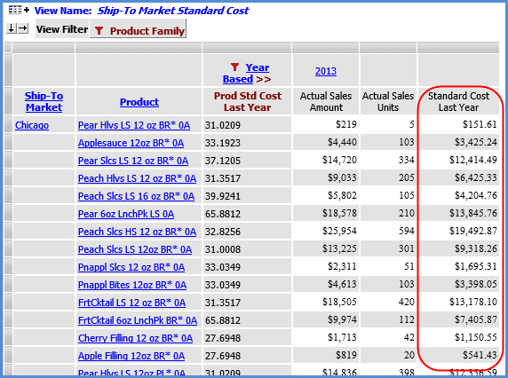
Standard Cost

Uses Val function and attribute relationship. IIF function checks for presence of the level to which attribute relationship belongs.

IIF([Product].[Product].CurrentMember.Level.Name="Product",Val([Product].[Product].Properties("Prod Std Cost Last Year"))*[Measures].[Data2 (Actual Sales Units)], null)

If the Product level is visible in the view, then the following calculation is performed:
Val([Product].[Product].Properties("Prod Std Cost Last Year"))*[Measures].[Data2 (Actual Sales Units)]. This returns the standard cost for last year and uses the Prod Std Cost Last Year attribute relationship multiplied by the Actual Sales Units to determine the results. If the Product level is not visible in the view, the calculation will not be performed and a null value (empty cell) will be returned.
The IIF and [Product].[Product].CurrentMember.Level.Name="Product" syntax check for the visibility of the level to which the attribute relationship belongs. The syntax for the measure item used in the expression includes its name (Data2) and caption.
Recommendation: select a monetary Format String.

Here is the view when the Product level is visible. The calculation is performed.

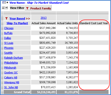
Here is the view when Ship-to Market has been drilled up to and Product is no longer visible. Null values are returned.

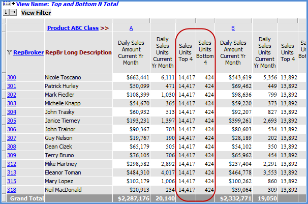
Top N Total

and

Bottom N Total

Use Sum function.

Sum({TopCount([RepBroker].[RepBroker].[RepBroker].members, 4, [Measures].[Data2 (Daily Sales Units Current Yr Month)])}, [Measures].[Data2 (Daily Sales Units Current Yr Month)])

and

Sum({BottomCount([RepBroker].[RepBroker].[RepBroker].members, 4, [Measures].[Data2 (Daily Sales Units Current Yr Month)])}, [Measures].[Data2 (Daily Sales Units Current Yr Month)])

The first calculation returns the total sales of the four RepBrokers with the highest sales. The portion of the expression enclosed in curly brackets { } and beginning with TopCount is what tells Stratum.Viewer to look for the four RepBroker members with the highest values for the specified measure item of Daily Sales Units Current Yr Month. The sum part of the expression is what totals the four values. The expression syntax includes the name of the RepBroker level, hierarchy, and dimension and includes the name (Data2) and caption of the measure item.
The second calculation returns the total sales of the four RepBrokers with the lowest sales. The calculation is set up the same as the first calculation except it uses the BottomCount function.
Recommendation: set Format String to the same Format String for the measure item referenced in the expression and set Total property to None.

Variance Percentage

Use the Percent of Change function when you want to include a variance percentage calculation in your view. That function is a Stratum.Viewer function that automatically includes a divide by zero check in the calculation to avoid divide by zero errors. See the first table in this topic for an example.

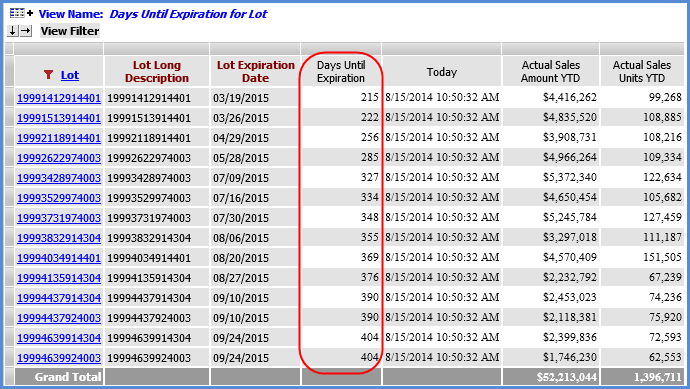
Days Until Expiration

Uses the Date Difference function in combination with the Today date function and an attribute relationship.

DateDiff("d", Now(), [Lot].[Lot].Properties("Lot Expiration Date"))

Returns the days until items expire, in this case, Lots. This calculation was built by selecting the Date Difference function, specifying "d" to calculate the difference in days, then selecting the Today function (which returned the Now() syntax), and finally selecting the Lot Expiration Date attribute relationship from the Lot level. The Date Difference and Today functions are in the VBA folder of the Expression window.
The current date in this case was August 15, 2014. The difference between that date and the Lot Expiration Date gives us the results in the Days Until Expiration date column in the example that follows.
Recommendations: leave the Format String set to None and set the Total property to None.

Notes: Results returned with negative numbers mean the expiration date has already been passed and it occurred the specified number of days ago. This example happens to calculate the "days" until expiration; therefore, it uses the parameter of "d" in the Date Difference function. Here are other parameters that can be used for calculations that involve other intervals of time: yyyy for year, q for quarter, m for month, y for day of year, d for day, w for weekday, ww for week, h for hour, m for minute, and s for second.